The Interpretability of AI: A Look into the Black Box of Machine Learning
A lot of manufacturers have already recognized that artificial intelligence (AI) offers enormous potential for medicine. But what if humans stop being able to follow the AI’s conclusions? This is a real and acute problem, which the concept of “AI interpretability” can help with.
The interpretability of machine learning ensures that AI-based (medical) devices do not become black boxes – and, in the worst-case scenario, endanger patients’ lives as a result. It enables errors to be identified and security vulnerabilities to be avoided.
In this article, you will learn:
- What interpretability of machine learning means
- What problems it solves and
- What methods can be used to achieve it
Note:
In sections 1 and 2, we provide an introduction to the subject that non-experts will be able to follow. Sections 3 and 4 concern specific methods for achieving machine learning model interpretability.
1. What does interpretability mean in the context of machine learning/AI?
a) Machine learning
Machine learning is a sub-discipline of artificial intelligence. It allows the computer to “learn” rules from data without it having to be explicitly programmed. In medical technology, machine learning is principally used for the processing of image and text data. “Deep learning” is often used for this. Deep learning means artificial neural networks that have a particularly high number of “layers.”
Further information
You can find out more about the basics of artificial intelligence and machine learning in our article on artificial intelligence in medicine.
b) Interpretability of machine learning
But what is meant by the interpretability of machine learning?
Definition: Explainability:
The degree to which a system can provide clarity about the reasons for its results (its outputs).
Example: For example, a procedure that evaluates the relevance of a machine learning model's features can increase the explainability of the model.
Definition: Transparency:
The degree to which a system reveals information about its inner workings, i.e., its internal structure and training data.
Explanation:
This means transparency is not the same as explainability. Explainability does not require the black box to be opened up. Transparency very much does. For example, a simple decision tree has high transparency because you can read the prediction of this model directly from the structure of the tree.
Definition: Interpretability:
The degree to which someone can use the information that the system provides as a result of its explainability and its transparency.
According to this definition, we can represent interpretability with an equation:
Interpretability = Explainability + Transparency
Therefore, the are two levers we can pull to improve interpretability in machine learning: explainability and transparency.
Transparency can be created by using inherently transparent models or methods that are applied after the AI has been trained.
Explainability can be achieved through numerous different approaches depending on the data type and question. This article introduces both concepts.
c) Why are machine learning models often so difficult to follow?
AI decision-making mechanisms depend on patterns in data. On the one hand, AI learns such patterns to mimic human abilities (for example, to detect objects in images). Conversely, thanks to AI, computers can recognize patterns that are not visible to humans. However, the models that result from this machine learning process are often very hard to follow.
This is mainly because the system creates these models itself using the data it learns with. The result of the computer's “learning process” is no longer programmed by a human.
These models are often extremely complex. In neural networks, for example, millions of parameters are trained.
Therefore, in a lot of cases, AI models are like black boxes – and even the people who developed them no longer understand them.
2. Avoid problems caused by a lack of AI interpretability
As powerful as AI can be, a lack of transparency and explainability can cause major errors to go undetected or even render the model unusable. In the worst-case scenario, this puts patients at risk.
a) Examples
How dangerous a lack of interpretability can be for patients is best illustrated by examples:
Dangers due to opaque models
A lack of transparency can lead to incorrect conclusions not being noticed by the manufacturer in time. Example: an AI model does not reliably detect cancer through suspicious lung tissue but (also) from the fact that the images were ordered by a specific person such as an oncologist.
Dangers due to unexplainable models
Sepsis Watch is a model that predicts sepsis in hospitalized patients based on clinical data. The model was integrated into clinical practice, where a rapid response team (RRT) nurse was responsible for the use of the tool. When alerted by the program, the RRT nurse notified the physicians on the ward. The method relied on deep learning without providing any additional explanation for the sepsis warning. This made communication more difficult (“But the patient looks well enough, why should they be at a high risk?” asked the doctors) and even led to RRT nurses trying to work out themselves why a particular prediction was made. The users thus created an “interpretability” for themselves, but it was often inaccurate.
(Reference: Repairing Innovation - A Study of Integrating AI in Clinical Care)
b) How interpretability solves problems and minimizes hazards
To avoid potential problems and minimize dangers, developers should ensure that their AI systems are interpretable. This will help them in several ways:
Finding errors during development
Not all errors lead to the model being of a low quality. Some errors, e.g., non-causal correlations already present in the data, can be detected through interpretability.
- Example – not direct causal factors: when asthma is wrongly used as a mitigating factor in pneumonia (even though the actual causal link is that asthma patients are prescribed antibiotics more quickly because they are a risk group. Therefore, the risk of asthma patients as a group dying from pneumonia is lower overall. There is more information in this paper).
- Example – biased results: AI that automatically assigns a low credit rating score to a specific ethnicity because it has learned through poor initial programming that minorities have lower incomes.
Detecting a model's limitations
Interpretability opens up the possibility of systematically dealing with how the model works. For example, if you notice that a tool for diagnosis relies mainly on the text of physicians’ reports (and less on blood values, visit data, etc.), it is reasonable to assume that the model will not work as well in a clinic where physicians’ reports are simply not available to the model because they are only available in analog form.
Identifying security gaps
Some risks can only be evaluated using interpretability. For example, adversarial attacks (attacks where the AI is tricked into malfunctioning through manipulated input) can reveal whether the model is vulnerable to attack.
Creating trust among all stakeholders
Interpretability can be used, for example, to synchronize the model’s way of working with expert knowledge in order to build a certain level of confidence.
Getting feedback to improve the model
This is especially true for the developers of the model. For example, if it becomes apparent that the model relies on particular features, it may be possible to improve these features specifically through feature engineering (to generate new, modified features).
If, for example, a particular blood value is an important feature, it may be possible to improve the prediction by using the evolution this blood value over time as a feature.
Obtaining evidence of performance and safety
If the systems are more comprehensible, the safety and performance of a device can also be demonstrated more effectively. This evidence is important for, e.g., notified bodies.
As explained above, transparency and explainability are needed to achieve the required level of interpretability.
3. Creating interpretability through transparency
Interpretability can be achieved through transparency. Again, there are two basic options:
- Transparency by design
This involves the use of inherently transparent models. You can restrict yourself, right from the start, to models that have an easily understandable and, therefore, transparent structure, such as decision trees and generalized additive models, or...
- Adding transparency later
With this option, models that are not intrinsically transparent are retrospectively made transparent using special methods. These make complex models, such as neural networks, interpretable by making their structure more transparent.
a) Transparency by desig
Generalized additive models
The name sounds very complicated, but ultimately generalized additive models (GAM) are mathematical formulas that calculate predictions based on the features. These formulas weigh and combine the features, learning the optimal value of the weights in the training process. A GAM is a transparent model because you can see directly from the formulas how the prediction is made.
Example:
The glomerular filtration rate (GFR) is an important indicator of kidney function (the lower it is, the worse the kidney function). However, GFR is difficult to measure. So, the ratio is estimated using features – this is then known as the eGFR. Several different formulas can be used. Here, for example, is the MDRD formula:
eGFR = 175 x SKr -1.154 x A -0.203
where SKr is serum creatinine and A is the patient's age. For women, the score is multiplied by 0.742 and, for Black people, by 1.212 (a factor that has already attracted harsh criticism). Researchers have used data to estimate the precise value for this weighting.
For example, using a bit of basic math, you can see just by looking at the formula that an increase in age, if all else remains the same, will result in a lower eGFR score.
Other examples of inherently interpretable models
- Decision trees: in the case of machine learning, these trees are not designed by hand. Instead, the “ramifications” are learned from the data. However, a white box can very quickly become a black box. For example, a very deep decision tree is difficult to follow.
- Decision rules are closely related to decision trees. A decision rule always follows the standard if-then construct: if certain feature values are present, a certain prediction is made.
b) Adding transparency later
Example of models that are not inherently interpretable
- A classic example of a black box model is a deep neural network (keyword: deep learning). They are generally not traceable and, therefore, fall into the black box model category.
- Another example is the random forest. As the name suggests, a random forest consists of trees, i.e., decision trees, that are considered intrinsically transparent. However, as the random forest consists of several hundred trees, it has to be categorized as a black box model – the transparency is lost as a result of the complexity.
Methods for more transparency
Transparency can also be increased for these black box models. However, this requires additional effort to interpret a model's individual components, for example, individual neurons in a neural network.
Example: feature visualization method
The feature visualization method is a good example of how transparency can be increased in convolutional neural networks (CNN). CNNs are used to classify images. What role the individual neurons play in this process is not immediately clear. The network is not transparent.
The feature visualization method can be used to systematically generate images that individual neurons in the network respond to in particular. This then enables us to better interpret how the model is working.
The following image shows the images that activate different neurons in the CNN. You can see that the neurons in the first level of the network principally recognize edges. The further back the level, the more complex shapes and structures can be recognized, up to and including objects such as dogs’ snouts.

Example: attention mechanisms
Attention mechanisms of certain neural networks are another example. These have internal weights that determine, for example, how much attention is paid to specific image regions or words when a classification or prediction is made. They can also be visualized to increase the transparency of these networks. However, there are still arguments about the extent to which these attention weights can be considered as interpretation (for more on this: Attention is not Explanation).
4. Interpretability through explainability
Another approach for ensuring the interpretability of AI is explainability. Its main advantage over transparency is that the black box doesn’t have to be opened. Explainability works only with inputs and outputs and leaves the underlying model untouched.
a) Feature effects
A feature effect describes how a single feature (e.g., the age of a patient) affects a model's output (e.g., cancer risk) on average. “On average” is important here because it is not about how the feature has affected an individual case but about how the model output behaves for the majority of data sets.
Feature effects can be visualized using graphs with the feature (e.g., age) on the horizontal axis and the model's prediction (e.g., cancer risk) on the vertical axis. The feature effect is then visualized by a curve.
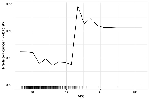
The graph shows an example of a feature effect plot. In this case, the partial dependence plot method has been used, but the graph would look very similar with other methods as well. We can see that as age increases, the probability of cancer decreases slightly. Around the age of forty, the probability of developing cancer rises sharply, then levels off again before remaining at a constantly high level from the age of sixty onwards. The dashes on the horizontal axis indicate the actual age observed in the data – almost no one was over the age of 50, so we shouldn’t overestimate the feature effect in this range.
Calculating the feature effect using the partial dependence plot
The partial dependence plot is calculated as follows: For example, you want to know the average effect of patient age on the probability of disease X as predicted by the model. In this case, you would start with the lowest age observed in the data, e.g., 20 years. Then you would artificially set the age of all patients in the data set to 20 and measure the average prediction for disease with this data set in the model. Then you repeat the whole process for age 21 and so on until you reach, e.g., 80. You have now simulated how the probability changes when the age is increased but all the other patient features remain the same.
There are other techniques for calculating feature effects: accumulated local effect plots, individual conditional expectation curves and Shapley dependence plots (but that would be going into too much depth here). Some of these are more complicated to calculate than the partial dependence plot described here but they work and are interpreted similarly.
b) Permutation feature importance
Permutation feature importance is a method that determines, for each of a model’s different input features, how important this feature was for correct predictions based on the data.
Concept
Permutation feature importance is based on a simple principle:
First of all, the model's performance is measured. Then, one of the features is permuted, i.e., the values in the corresponding table column are randomly shuffled. This “destroys” the connection between this feature and the correct prediction. The model’s performance is then re-measured using this “incorrect” data. If the feature has no effect on the prediction, the performance will be unaffected. If the model relies heavily on this feature to make a correct prediction, the performance will decrease significantly. Repeating this procedure for all features provides a ranking of the importance of each feature.
It may already be clear from the description why this method can also be used to explain black box models: it works simply by “manipulating” the model's input data and measuring the change in the output. No model transparency is required.
Example
Model for predicting the development of hypertension later in life based on cardiorespiratory fitness data.
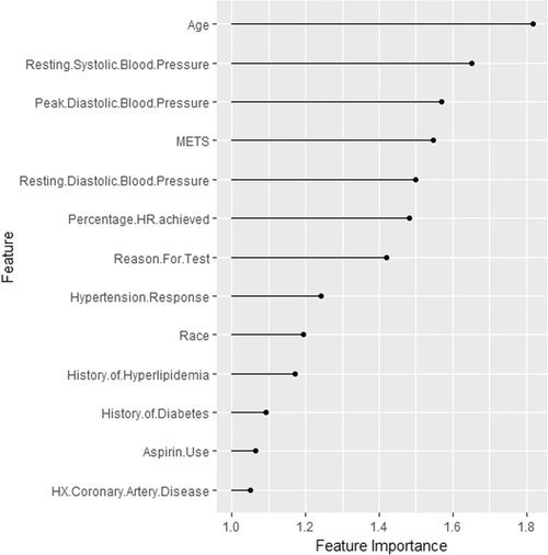
We can see here, for example, that age was the most important feature. This is followed by features such as resting systolic blood pressure and peak diastolic blood pressure. This information can now be synchronized with expert knowledge. We now know that age is an important factor for the model. It may make sense to look at the model's performance broken down by age.
c) Shapley values
The Shapley values explanation method that can explain the prediction for individual data points. In this method, the prediction is “fairly” distributed across the individual features to explain how the model's predictions were arrived at.
Concept
Shapley values actually come from game theory: suppose that some players play a cooperative game and receive prize money. How should this prize money be divided fairly between the players? The Shapley value method offers a solution to this problem. First, all possible combinations of players are simulated, including the resulting prize money. Then each combination is compared: what is the prize money with or without this player? The average difference in prize money is then that player's fair share.
The principle can also be applied to machine learning: The “players” are the individual feature values for a given data set. The “prize money” is the model's prediction, which must be divided fairly among the feature values. There is one more nuance to consider: It is not the prediction as a whole that is divided, but the difference to the mean prediction with the whole data set. Therefore, the Shapley values can be used to interpret why exactly this data set has a different prediction compared to the data set for the mean.
Use
Shapley values can be used in a range of fields: they can be used for image and text data as well as table data. Furthermore, Shapley values (at least when applied to table data) can be aggregated across data sets. This means they also allow interpretation of the overall distribution of the model's data, e.g., with regard to feature effects and the importance of features.
Example
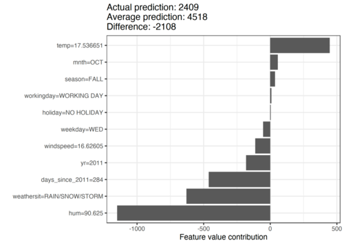
In the following example, a machine learning model that predicts the number of bicycles rented daily from a bike rental company has been trained. Calendar information, such as the month and day of the week, and the weather were used as features. The aim now is to explain the prediction of 2409 bicycles on a particular rainy day in October. It is 2108 bicycles below the average prediction. We can see that the high humidity of 90% and the rainy weather were mainly responsible for this low forecast. However, the temperature of 17 degrees was also a factor in the prediction – in this case, a positive factor. If you add the Shapley values for the features together, you get the difference of -2108.
d) Counterfactual explanations
Counterfactual explanations are “what-if” explanations that show what feature values would have to have been changed for the machine learning model to have come to a different prediction. Similar to Shapley values, this method is also suitable for the prediction of individual data points.
Concept
For counterfactual explanations, the prediction must be selected by the user. For example, if a diagnosis tool says that a patient probably has cancer, counterfactuals would be generated for the opposite classification of “no cancer”: a counterfactual explanation could be, for example, that if a certain blood value was lower, the diagnosis would be “healthy.”
There are a wide range of algorithms for finding counterfactual explanations. However, theoretically a human can also create counterfactuals by, for example, “playing” with the inputs to an AI tool to try to change the output. Counterfactual explanations are thus easier to understand, even for non-experts. However, it is always possible to create any number of counterfactual explanations for a model's prediction.
Example
Credit score: A person with certain attributes (age, sex, job, housing, savings) wants a certain amount of credit, for a certain amount of time and for a specific reason.
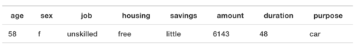
The model calculates the probability that the credit will be repaid.
According to the model, there is a 24% chance that the person will repay the credit. What would have to be different for this probability to be at least 50%?
Here are two different counterfactuals:
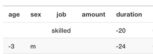
the job plays the most important role. For example, if the customer were in a “skilled” job and the length of the loan was 20 months shorter, the credit score would be higher. Or if she were a man and three years younger, and the credit duration 2 years shorter, she (or he) would have been given the loan. This latter example also shows that this algorithm discriminates against women.
e) Saliency maps: LRP, GradCAM, integrated gradient and Co.
Saliency maps highlight regions in images that are important for predictions by image recognition algorithms based on deep learning.
Concept
Saliency maps are very useful for understanding why the model learned the wrong thing. There are a lot of examples, particularly from medicine, where it became apparent that the model has learned “shortcuts” that are ultimately not helpful. However, these errors were not evident in the model's performance.
Example
The analysis of images taken for skin cancer predictions: saliency maps can be used to show, for example, that a neural network uses markings made by the physician themselves with a pen or overlaid rulers in images to classify melanomas. Obviously, this is far from ideal. This is because an assessment by the physician is being included indirectly. Suspicious areas are more likely to be marked and measured than non-suspicious ones.
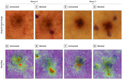
Association Between Surgical Skin Markings in Dermoscopic Images and Diagnostic Performance of a Deep Learning Convolutional Neural Network for Melanoma Recognition - https://jamanetwork.com/journals/jamadermatology/fullarticle/2740808
Saliency maps are very useful for detecting errors. This is especially true during the development process. There are a huge number of methods in this category: for example, LRP, GradCAM, vanilla gradient, integrated gradient, DeepLift, DeepTaylor etc. What the methods have in common is that they use the gradients (i.e., the mathematical derivative) of the model prediction with respect to the input pixels. Or, to put it more simply: you measure how sensitive the model prediction is to changes in pixels. The more sensitive it is, the more important the pixel. Some methods also differentiate between whether a change in pixel intensity changes the prediction negatively or positively. Saliency maps themselves are images that are overlaid over the images being classified in order to mark the locations that are important for the prediction.
f) Other methods specific to deep learning
- Adversarial attacks:
These are special data sets that look normal to humans, but which lead to misclassifications when used in models. For example, you can make slight changes to the pixels on images. The image still looks the same to a human, for example, you still see a dog. But the model now classifies the images incorrectly.
- Influential instances:
This technique can be used to identify the training data sets that were the most relevant to the neural network classification or prediction.
This article only offers a first impression of the available techniques. The variety of methods out there is much higher and only time will tell which ones emerge as the standards.
5. Regulatory considerations
European medical device law does not establish any specific requirements for the use of artificial intelligence or even the interpretability of models. However, medical device law does require the following from manufacturers:
- Development according to the state of the art
- The best possible benefit-risk ratio
- Safe devices
- The results to be repeatable
The methods described above represent the state of the art. They help to detect hazards and thus minimize risks and improve the benefit-risk ratio.
From this, we can deduce that machine learning-based medical devices that ignore interpretability methods do not correspond to the state of the art. This is true at least for those medical devices whose ML models have an impact on their safety, performance and clinical benefit.
6. Conclusion
Machine learning has arrived in the medtech industry due to its high performance levels. This is especially true for image and text recognition. The FDA and European authorities have already authorized such systems. We should expect machine learning to play an increasingly key role in the medtech industry in the future.
But this could also lead to problems: AI whose models are no longer comprehensible can be dangerous for patients. Manufacturers should take steps to counteract any potential problems at an early stage of development. Interpretability methods are one way of doing this.
Interpretability is as useful during the development phase as it is during the post-market surveillance phase. In both these phases, manufacturers should pay close attention to how well the method works – and whether end users can understand the explanation.
This article was initially written by Christoph Molnar, an expert on interpretability in machine learning. His book Interpretable Machine Learning is available on his website.

Author:
Heidi Seibold

Back To Top
Privacy settings
We use cookies on our website. Some of them are essential, while others help us improve this website and your experience.